Spectral Instability in Attention Matrices as a Leading Indicator of Transformer Rule Violations

Code and data: github.com/ParkerWilliams/dcsbm-transformer

Motivation: Why a Controlled Setting

Studying how transformers fail in production is hard. When a language model hallucinates during summarization or loses track of a fact mid-generation, the failure involves thousands of interacting variables: document structure, entity density, training data coverage, decoding strategy. Isolating the mechanism is nearly impossible because ground truth is ambiguous and the internal state is enormous.

We need a setting where the model must maintain latent constraints over variable distances, where we know exactly when it succeeds or fails, and where we can measure the full internal state at every step. This motivates a synthetic approach, not as an end in itself, but as a first-principles investigation before moving to production models.

The specific question: can spectral properties of the attention matrices predict when a transformer is about to fail, before the failure occurs? And if so, how far in advance?

The model I am using here is small and synthetic, and what I find will likely not transfer directly to a production system. My next piece of work is to take whatever principles emerge from this controlled setting and test them on Phi-3. This post is not a finished result. It is an honest look at where the investigation stands, after dozens of revisions to the experimental design, so that the reasoning is visible as the project moves forward.

At a high level, we are asking questions about the geometry of attention heads over time, reaching into a bag of tricks from random matrix theory and functional analysis, and asking whether any of it tracks with model failure.

Why DCSBM Graphs

A degree-corrected stochastic block model (DCSBM) defines communities of vertices with dense within-community edges and sparse between-community edges. Edge probabilities follow

\[ P_{ij} = \theta_i \, \theta_j \, \omega_{b_i, b_j} \]

where \(\omega_{ab} = p_{\text{in}}\) if \(a = b\), \(\omega_{ab} = p_{\text{out}}\) otherwise, and \(\theta_i\) are degree-correction parameters sampled from a Zipf distribution. This is a natural model of concept adjacency. Semantically related tokens are more likely to co-occur, and the block structure captures the clustering of concepts into topics or domains. The degree correction adds realistic heterogeneity: some vertices are hubs, others are peripheral, mirroring the power-law frequency distributions of natural language.

Training a transformer to predict next tokens on random walks over this graph forces it to learn community structure from sequential observations. The model must internalize which vertices tend to follow which, and how transition probabilities shift depending on the current block. This is analogous to how language models learn that certain tokens are likely in certain contexts.

The critical addition is block jumper vertices. Each jumper carries a delayed rule: encountering it at step \(t\) means the walk must reach a specific target community at step \(t + r\). By varying \(r\) across the set

\[ r \in \left\{ \lfloor s \cdot w \rceil \;\middle|\; s \in \{0.5,\, 0.7,\, 0.9,\, 1.0,\, 1.1,\, 1.3,\, 1.5,\, 2.0\} \right\} \]

where \(w\) is the context window, we control the difficulty of the constraint. Short rules (\(r = 32 = 0.5w\)) are easy because all relevant information is nearby. Long rules (\(r = 128 = 2w\)) are hard because the model must maintain a constraint that has long since left the attention window.

This maps directly to factual dependencies in language. A document states a fact on page one that constrains what can be said on page three. The model saw the constraint, but can it hold onto it long enough to act on it correctly?

The key property of this setup: every rule event has a known outcome (followed or violated), a known rule length, and a fully observable attention state at every intermediate step.

Experimental Setup

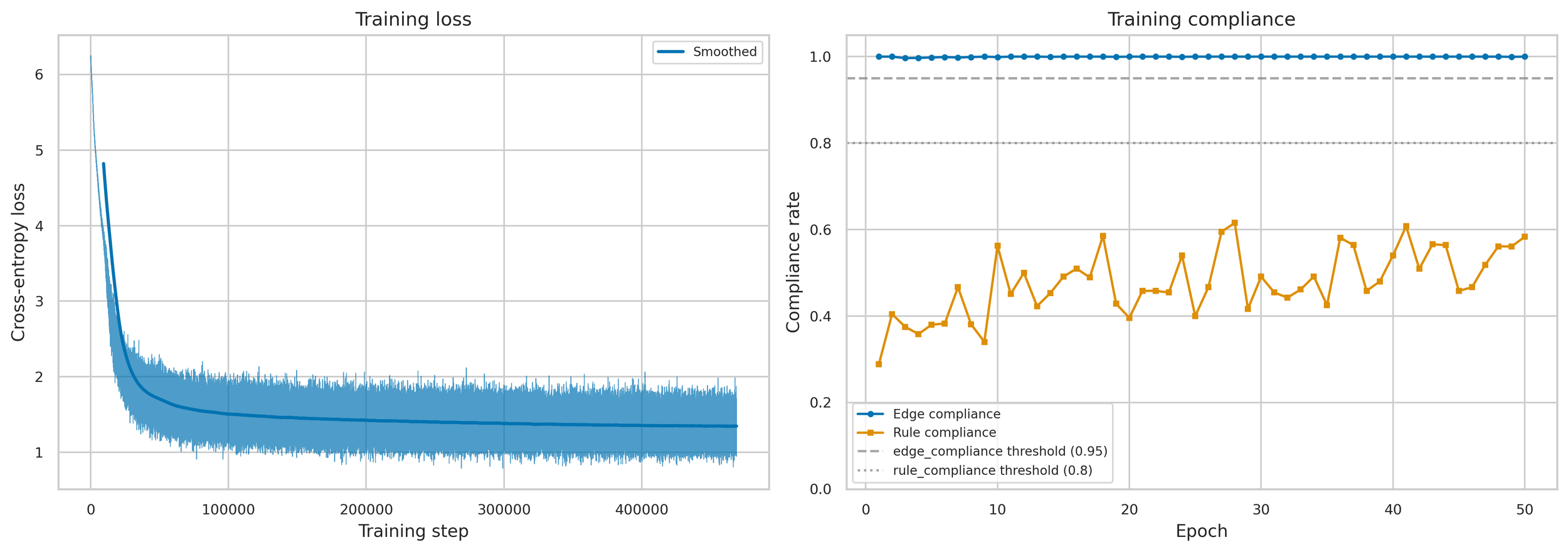
he anchor experiment uses a 4-layer, 1-head transformer with \(d_{\text{model}} = 128\) and a context window of \(w = 64\) tokens. The graph has \(n = 500\) vertices in \(K = 4\) blocks, with \(p_{\text{in}} = 0.25\) and \(p_{\text{out}} = 0.03\). Training runs for 50 epochs on 200,000 walks with next-token prediction, gated by a sufficiency criterion requiring edge compliance above 0.95 and rule compliance above 0.80 before proceeding to evaluation.

The model learns the local graph structure almost perfectly (edge compliance near 100%) but learns the delayed jumper rules only partially. Overall rule compliance plateaus around 55-60%, but this average masks wide variation by rule length. At \(r = 58\) (just below the context window), compliance reaches roughly 78%. At \(r = 83\) (just above), it falls to around 52%. The model is not ignorant of the rules. It is partially tracking the constraints and sometimes losing them, with the failure rate depending on how far the rule stretches relative to the context window. This is the regime we want: a model that has learned something real but fails often enough to study the failure mechanism.

At every generation step during evaluation, we compute the full SVD of both the \(QK^T\) attention matrix (the raw attention scores) and the \(A \cdot V \cdot W_O\) matrix (the attention-value-weighted output, which captures the OV circuit). From these decompositions we extract five spectral metrics:

Stable rank, defined as

\[ \text{srank}(M) = \frac{\|M\|_F^2}{\|M\|_2^2} = \frac{\sum_i \sigma_i^2}{\sigma_1^2} \]

This measures the effective dimensionality of the attention pattern. A matrix with one dominant singular value has stable rank near 1; a matrix with many comparable singular values has high stable rank.

Grassmannian distance, the geodesic on the Grassmannian \(\text{Gr}(k, n)\) between the top-\(k\) left singular subspaces at consecutive timesteps:

\[ d_G(U_t, U_{t-1}) = \left\| \arccos\left(\sigma_i(U_t^T U_{t-1})\right) \right\|_2 \]

This measures how fast the attention subspace rotates from one step to the next.

Spectral entropy, defined as

\[ H = -\sum_i p_i \log p_i \quad \text{where} \quad p_i = \frac{\sigma_i}{\sum_j \sigma_j} \]

This measures how uniformly the singular values are distributed.

These are measured on both \(QK^T\) and \(AVWO\), giving complementary views into the attention mechanism (what the model is attending to) and the output circuit (what information is being written).

The evaluation produces 22,222 sequences with 211,729 total rule events across 8 rule lengths: \(r \in \{32, 45, 58, 64, 70, 83, 96, 128\}\).

Result 1: Spectral Instability Precedes Violations With Long Horizons

Before presenting AUROC numbers, the most important thing to communicate about these results is that the measured effect sizes are very small. The mean difference between violation and control spectral traces is often less than 1% of the baseline value. If you looked at a single token's stable rank and tried to decide "violation or control," you could not do it. We are nowhere near having a threshold you could set on any one metric to flag failures in real time.

What we do find is that this small, per-step shift is statistically consistent. Across tens of thousands of events, it accumulates into a reliable rank-ordering between violation and control populations, which is what AUROC measures. This is a population-level statistical signal, not a per-token diagnostic.

With that caveat up front: for each metric and rule length, we compute AUROC at every lookback distance \(j\) from 1 to \(r\) steps before the rule resolution:

\[ \text{AUROC}(j) = P\!\left(X_{\text{violated}}^{(t-j)} > X_{\text{followed}}^{(t-j)}\right) \]

The predictive horizon is the maximum \(j\) where \(\text{AUROC}(j) > 0.75\).

Within a single rule-length regime, AUROC ranges from 0.75 to 0.98, and the predictive horizons scale with rule length:

At \(r = 32\) (half the window), \(QK^T\) grassmannian distance reaches 0.797 AUROC with a 17-step horizon.

At \(r = 45\) (\(0.7w\)), \(QK^T\) stable rank reaches 0.982 AUROC with a 27-step horizon.

At \(r = 64\) (exactly the window), AVWO grassmannian distance reaches 0.987 AUROC with a 64-step horizon.

At \(r = 96\) (\(1.5w\)), \(QK^T\) stable rank reaches 0.899 AUROC with a 95-step horizon.

At \(r = 128\) (\(2w\)), \(QK^T\) grassmannian distance reaches 0.946 AUROC with a 93-step horizon.

The attention subspace becomes measurably unstable well before the model emits the incorrect token. At \(r = 64\), the signal spans the entire rule length. But "measurably" here means detectable with enough data, not visible to the naked eye on a single sequence.

The event-aligned plots illustrate this honestly. These show the average metric value in a window around each rule event, with violations in orange and controls in blue.

Event-aligned \(QK^T\) stable rank. The violation trace (orange) runs slightly higher than the control trace (blue), but the separation is small in absolute terms: roughly 0.01 on a baseline of 1.49. The confidence bands overlap across the entire window. You would not look at this plot and conclude "these populations are cleanly separable." The AUROC is high because this tiny shift is consistent across 93,000 violation events and 118,000 control events, not because any individual token is diagnosable.

Result 2: Pooling Across Rule Lengths Destroys the Signal

Here is the central finding. We compute the same metrics, on the same data, but pooled across all 8 rule lengths. The AUROC drops to approximately 0.70 for the best single metric. We then test whether accumulating the signal over time recovers it:

Single raw metric (\(QK^T\) stable rank, lookback = 5): 0.700 AUROC pooled.

Rolling mean (window = 10) of stable rank: 0.700 AUROC pooled.

Rolling variance, CUSUM, EWMA deviation: 0.55 to 0.63 AUROC pooled.

5-metric logistic regression: 0.711 AUROC pooled.

Nothing breaks 0.72 when pooled. The cumulative metrics do not rescue the signal. Multi-metric composites add negligible lift.

The mechanism is straightforward. Different rule lengths place the model in qualitatively different spectral operating regimes. A model tracking a 32-step dependency has a different baseline stable rank than one tracking a 128-step dependency. The between-regime variation in baseline metric levels is larger than the within-regime violation-vs-control shift. Pooling mixes these regimes, and the regime differences dominate.

This is likely why prior approaches to spectral hallucination detection have reported weak results. If you measure attention-based features across a diverse set of inputs and correlate with output quality, you are implicitly pooling across what are effectively different operating regimes.

Result 3: Per-Regime Composites Recover Near-Perfect Discrimination

Conditioning on rule length and combining metrics changes the picture entirely. We fit a logistic regression on 5 raw spectral metrics (\(QK^T\) stable rank, \(QK^T\) grassmannian distance, \(QK^T\) spectral entropy, AVWO stable rank, AVWO grassmannian distance) evaluated within each rule-length stratum at a lookback of 5 steps:

\(r = 32\) (\(0.5w\)): 0.79 composite AUROC. Best single metric avwo.gd at 0.77.

\(r = 45\) (\(0.7w\)): 0.96 composite AUROC. Best single metric qkt.sr at 0.88.

\(r = 58\) (\(0.9w\)): 0.86 composite AUROC. Best single metric avwo.sr at 0.72.

\(r = 64\) (\(1.0w\)): 0.95 composite AUROC. Best single metric avwo.sr at 0.85.

\(r = 70\) (\(1.1w\)): 1.00 composite AUROC. Best single metric qkt.gd at 0.92.

\(r = 83\) (\(1.3w\)): 0.78 composite AUROC. Best single metric qkt.sr at 0.67.

\(r = 96\) (\(1.5w\)): 0.94 composite AUROC. Best single metric qkt.sr at 0.93.

\(r = 128\) (\(2.0w\)): 0.89 composite AUROC. Best single metric qkt.gd at 0.86.

Seven of eight regimes exceed 0.86 AUROC with the composite. The pattern holds across lookbacks from 1 to 20 steps.

Critically, no single metric dominates across regimes. \(QK^T\) stable rank carries \(r = 45\) and \(r = 96\). \(QK^T\) grassmannian distance carries \(r = 70\) and \(r = 128\). AVWO stable rank carries \(r = 58\) and \(r = 64\). AVWO grassmannian distance is the strongest contributor at \(r = 32\) where everything else is mediocre. The composite works because the metrics are genuinely complementary, each sensitive to a different failure geometry.

The one difficult regime is \(r = 83\) (\(1.3w\)). This is where the jumper encounter falls just inside the context window but resolution is well outside. The model has partial information about the constraint, and the spectral signature of that partial knowledge is the hardest to distinguish from normal operation. This finding is itself informative: it identifies the specific boundary condition where monitoring is weakest.

Interpretation: Regime-Dependent Monitoring

The three-layer result (strong per-\(r\), weak pooled, strong composite per-\(r\)) points to a specific architectural requirement for practical monitoring. The detector must calibrate to the current operating regime.

Two candidate approaches follow from this:

Self-calibrating change-point detectors. Algorithms like CUSUM and BOCPD establish a local baseline from the sequence's own history and flag deviations from it. They do not require knowing the regime explicitly. In our data, CUSUM on AVWO stable rank achieves 0.967 AUROC at \(r = 70\) without any knowledge of \(r\). It simply detects "something changed relative to what came before." The limitation is inconsistency: CUSUM works well at some rule lengths and poorly at others.

Explicit stratification. If the task structure is known (document length, dependency span, query type), per-stratum decision boundaries can be learned. This is more engineerable but requires task-specific calibration.

A note on computational cost: stable rank requires only \(\|M\|_F\) plus \(\sigma_1(M)\) (a few power iterations), not a full SVD. Grassmannian distance needs the top-\(k\) singular vectors, achievable via truncated or randomized SVD. A practical monitoring system can run these cheaply at inference time, reserving full spectral analysis for flagged regions.

Where This Goes: Phi-3-mini and Inter-Head Geometry

To be direct about what this is and what it is not. This is a result on a toy model in a controlled setting. The transformer is tiny. The task is synthetic. Real language involves many overlapping dependencies of different lengths operating simultaneously, not one clean rule resolving at a known step. The regime-conditioning result could be an artifact of the simplicity of the setup, where there is exactly one rule length per event and nothing else competing for the model's attention.

What the result does give us is direction. It tells us which spectral properties of attention are worth measuring, it tells us that regime-dependence is a specific threat to detection quality that needs to be addressed rather than ignored, and it tells us that complementary metrics on different circuits (QKT vs AVWO) contribute genuinely different information. These are design principles for the next experiment, not conclusions about production systems.

The next step is Phi-3-mini (3.8B parameters, 32 heads, 32 layers) on tasks where we can evaluate output quality against ground truth. Document QA with controlled evidence distance is one candidate, where the distance from question to supporting evidence serves a role analogous to \(r\). Summarization faithfulness is another. The question is whether the spectral signatures we observed here show up at all in a model that is 30,000x larger and operating on natural language rather than graph walks.

Phi-3-mini also opens up a measurement that was unavailable here: inter-head geometry. With 32 attention heads per layer, we can compute the Grassmannian distance between head \(i\) and head \(j\)'s \(QK^T\) subspaces at the same token, \(d_G(U_t^{(i)}, U_t^{(j)})\). This measures whether heads that normally agree are diverging. In the DCSBM experiment, the composite worked because different metrics on a single head captured different failure geometries. With multiple heads that specialize in different dependency types, the pairwise relationships between their subspaces may carry richer information about the model's internal state than any single-head metric can provide. That is a hypothesis, not a result. Testing it is the next piece of work.

The full codebase, data, and analysis scripts are available at github.com/ParkerWilliams/dcsbm-transformer.